A first OP example

Performing numeric Operating Point (OP) simulations with ahkab of linear networks – like those in undergrad network theory textbooks– is really straight-forward.

The circuit

In this brief text, we will describe the following circuit:

Circuit description

First of all, we need the ahkab library to be imported:

import ahkab

Next, we create a new circuit object. The only parameter you need is the name, which in the following is ‘Simple Example Circuit’.

mycir = ahkab.Circuit('Simple Example Circuit')

Now’s time to add the elements. The circuit object we just created (mycir) offers plenty of convenience methods to add elements to your circuit instances.

The general structure of the methods signature is:

add_<element_type>(part_id, node1, node2, value)

For example, we have an add_resistor method, with signature:

add_resistor(part_id, n1, n2, value)

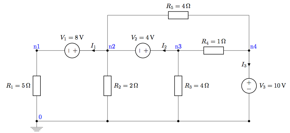
Our circuit is described by:

mycir.add_resistor('R1', 'n1', mycir.gnd, value=5)
mycir.add_vsource('V1', 'n2', 'n1', dc_value=8)
mycir.add_resistor('R2', 'n2', mycir.gnd, value=2)
mycir.add_vsource('V2', 'n3', 'n2', dc_value=4)
mycir.add_resistor('R3', 'n3', mycir.gnd, value=4)
mycir.add_resistor('R4', 'n3', 'n4', value=1)
mycir.add_vsource('V3', 'n4', mycir.gnd, dc_value=10)
mycir.add_resistor('R5', 'n2', 'n4', value=4)

Defining the simulation and running it

Next, we need the OP simulation object. And then we start the simulation.

opa = ahkab.new_op()
r = ahkab.run(mycir, opa)['op']

The simulation takes a few milliseconds.

Inspecting the results

Simply printing the results with print formats the simulation results in a nice table:

print r

OP simulation results for 'Simple Example Circuit'.
Run on 2015-05-09 12:38:54, data file /var/folders/9y/nry2qj0962l38pqk3_8_8ndm0000gn/T/tmpiF4Jvs.op.
Variable    Units        Value         Error    %
----------  -------  ---------  ------------  ---
VN1         V        -3.86364    3.86369e-12    0
VN2         V         4.13636   -4.13614e-12    0
VN3         V         8.13636   -8.13571e-12    0
VN4         V        10         -1.00027e-11    0
I(V1)       A        -0.772727   0              0
I(V2)       A        -0.170455   0              0
I(V3)       A        -3.32955    0              0

The op_solution class also provides an easy to use dictionary-like interface to access your data, which is described in the documentation.

Conclusions

We hope this example, while basic, allows you to get more confident with using ahkab, especially to simulate linear networks.

Don’t forget to report any bugs you may run into – it happens! – and have fun doing electronics! :)