Transient example
Introduction
This is an example of transient simulation, featuring the well-known Colpitts oscillator.
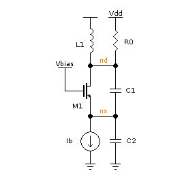
Bias:
\(V_{dd}=2.5V\), \(V_{bias}=2V\).
Passives:
\(L_1 = 5 nH\), \(R_0=3.14 k\Omega\) (\(Q_L=33\) @ 3 GHz)
\(C_1 = C_2 = 1.012 pF\) (resulting in \(n = C_1/(C_1 + C_2) = 0.5\))
\(C_2\) has a \(Q\) greater than 10 for every \(I_b\) less than \((w_0 C_2)^2/(2 K 10^2)\) = 4.8 mA.
Under such condition, the minimum transconductance required for oscillation can be calculated considering the MOS transistor an ideal voltage probe. The presence of the MOS has to be taken into account when evaluating the overall \(Q\) of the tank.
Under such hypothesis: \(g_{m,min} = 1/(n(1-n)R0)\), \(I_{b,min} = 1.27\) mA. In the following we use \(I_b\) = 1.3mA.
Netlist-based simulation
Netlist
MOS COLPITTS OSCILLATOR

vdd dd 0 type=vdc vdc=2.5

* Ql = 33 at 3GHz
l1 dd nd 5n ic=-1n
r0 nd dd 3.5k

* n = 0.5, f0 = 3GHz
c1 nd ns 1.12p ic=2.5
c2 ns 0  1.12p *ic=.01

m1 nd1 bias ns ns nmos w=200u l=1u
vtest nd nd1 type=vdc vdc=0 *read current

* Bias
vbias bias 0 type=vdc vdc=2
ib ns 0 type=idc idc=1.3m

.model ekv nmos TYPE=n VTO=.4 KP=10e-6

.op
.tran tstop=150n tstep=.1n method=trap uic=2
.plot tran v(nd)
The voltage generator Vtest has been added to the circuit in series with M1’s drain to add the drain current to the variables.
We need to simulate the circuit for roughly \(T \approx 10Q_L/f_0\) = 110ns to approach the steady state solution. The simulation above stops at \(t\) = 150ns.
Running the simulation
Save the netlist in a file and start ahkab with:
$ ahkab colpitts_mos.spc -o colpitts_graph
The simulation takes 70s on my laptop. Set tstop to a lower value to make it
faster.
Results
Operating point (.OP)
The operating point is shown in this section of the program output:
2015-02-23 15:28:37
ahkab v. 0.13 (c) 2006-2015 Giuseppe Venturini

Operating Point (OP) analysis

Netlist: colpitts_mos.ckt
Title: MOS colpitts oscillator
At 300.00 K
Options:
    vea = 1.000000e-06
    ver = 0.001000
    iea = 1.000000e-09
    ier = 0.001000
    gmin = 0.000000e+00

Convergence reached in 42 iterations.

========
RESULTS:
========

Variable        Value         Error  (%)      Units
----------  ---------  ------------  -------  -------
VDD          2.5       -2.5e-12      (-0.00)  V
VND          2.5       -2.5e-12      (-0.00)  V
VNS         -0.116201   2.48567e-10  (-0.00)  V
VND1         2.5       -2.50951e-10  (-0.00)  V
VBIAS        2         -2e-12        (-0.00)  V
I(VDD)      -0.0013     0            (-0.00)  A
I(L1)        0.0013     0            (0.00)   A
I(VTEST)     0.0013     0            (0.00)   A
I(VBIAS)     0          0            (0.00)   A

========================
ELEMENTS OP INFORMATION:
========================

Part ID      V(n1-n2) [V]         Q [C]        E [J]
---------  --------------  ------------  -----------
C1               2.6162     2.93015e-12  3.83292e-12
C2              -0.116201  -1.30145e-13  7.56149e-15

Part ID      V(n1-n2) [V]    I [A]         P [W]
---------  --------------  -------  ------------
IB              -0.116201   0.0013  -0.000151061

Part ID      ϕ(n1,n2) [Wb]    I(n1->n2) [A]      E [J]
---------  ---------------  ---------------  ---------
L1                 6.5e-12           0.0013  4.225e-15

----  --------  -----------------  ----  ----  -----------------  -----  --------  -------------------------  ----  --------  -----------------
m1    N ch      STRONG INVERSION               LINEAR
beta  [A/V^2]:  0.000746574470194  Weff  [m]:  0.0002 (0.0002)    Leff   [m]:      1.33945110625e-06 (1e-06)  M/N:            1/1
Vdb   [V]:      2.616200987        Vgb   [V]:  2.116200987        Vsb    [V]:      0.0                        Vp    [V]:      1.18126783831
VTH   [V]:      0.4                VOD   [V]:  1.61188671993      nq:              1.44011732737              VA    [V]:      1.99917064176
Ids   [A]:      0.00129999988445   nv:         1.36453957998      Ispec  [A]:      3.84987888131e-06          TEF:            0.063129029685
gmg   [S]:      0.00184989038878   gms   [S]:  -0.00317451824956  rob    [Ω]:      1537.82370727
if:             475.729938341      ir:         23.4335578457      Qf     [C/m^2]:  0.00111108138735           Qr    [C/m^2]:  0.000227594358407
----  --------  -----------------  ----  ----  -----------------  -----  --------  -------------------------  ----  --------  -----------------

Part ID      R [Ω]    V(n1,n2) [V]    I(n1->n2) [A]    P [W]
---------  -------  --------------  ---------------  -------
R0            3500               0                0        0

Part ID      V(n1,n2) [V]    I(n1->n2) [A]     P [W]
---------  --------------  ---------------  --------
VDD                   2.5          -0.0013  -0.00325
VTEST                 0             0.0013   0
VBIAS                 2             0        0
Transient simulation (.TRAN)
The oscillation builds up quickly, as shown in this plot of \(V_{nd}\):
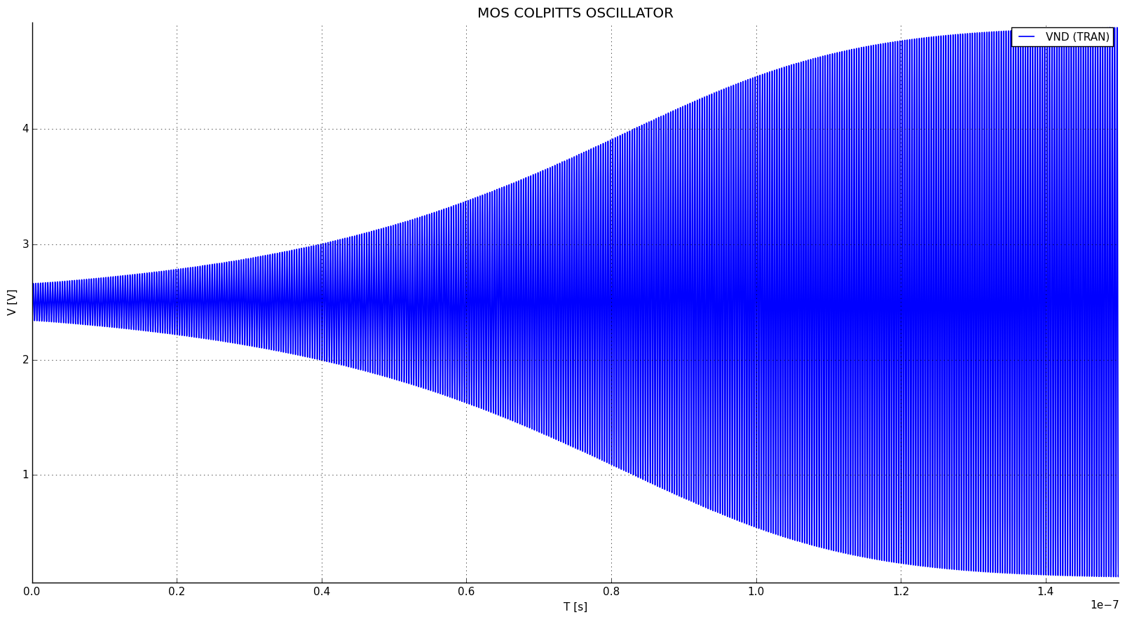
From inspection, the circuit oscillates at 3.002 GHz with an oscillation amplitude of roughly 4V.
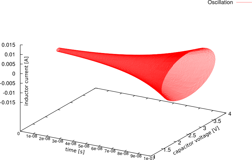
The next plot shows the oscillation starting off from the very beginning in a phase plane:
API-based simulation
As an exercise, we will show here also how to perform a similar simulation taking advantage of the Python API.
Python script
import ahkab
import pylab

osc = ahkab.Circuit('MOS COLPITTS OSCILLATOR')

# models need to be defined before the devices that use them
osc.add_model('ekv', 'nmos', dict(TYPE='n', VTO=.4, KP=10e-6))

osc.add_vsource('vdd', n1='dd', n2=osc.gnd, dc_value=3.3)

# Ql = 33 at 3GHz
osc.add_inductor('l1', n1='dd', n2='nd', value=5e-9, ic=-1e-9)
osc.add_resistor('r0', n1='nd', n2='dd', value=3.5e3)

# n = 0.5, f0 = 3GHz
osc.add_capacitor('c1', n1='nd', n2='ns', value=1.12e-12)
osc.add_capacitor('c2', n1='ns', n2=osc.gnd, value=1.12e-12)

osc.add_mos('m1', nd='nd1', ng='bias', ns='ns', nb='ns',
            model_label='nmos', w=600e-6, l=100e-9)
# voltage source as a current probe
osc.add_vsource('vtest', n1='nd', n2='nd1', dc_value=0)

# Bias
osc.add_vsource('vbias', n1='bias', n2=osc.gnd, dc_value=2.)
osc.add_isource('ib', n1='ns', n2=osc.gnd, dc_value=1.3e-3)

# calculate an Operating Point (OP) to initialize the transient
# analysis
op = ahkab.new_op()
res = ahkab.run(osc, op)

# modify the OP to give the circuit a little kick to start the
# oscillation
x0 = res['op'].asmatrix()
l1vdei = osc.find_vde_index('l1')
l1i = len(osc.nodes_dict) - 1 + l1vdei
x0[l1i, 0] += -1e-9

# Setup and run a transient analysis with the modified x0 as start point
tran = ahkab.new_tran(tstart=0., tstop=20e-9, tstep=.01e-9, method='trap',
                      x0=x0)
res = ahkab.run(osc, tran)['tran']

# plot the results!
pylab.subplot(211)
pylab.hold(True)
pylab.plot(res.get_x(), res['vnd'], label='ND')
pylab.plot(res.get_x(), res['vns'], label='NS')
pylab.plot(res.get_x(), res['vbias'], label='BIAS')
pylab.legend()
pylab.subplot(212)
pylab.plot(res.get_x(), res['i(vtest)'], label='I(VTEST)')
pylab.legend()
pylab.show()
As we have increased in the above the W of M1 and therefore its \(g_m\),
the oscillation will build up faster and to a higher top amplitude.
Running the simulation
To run the simulation, just save the above code to a file, for example
colp.py and run:
python colp.py
If matplotlib is available and set up correctly, a graph should pop up in a
little while.
Results
The OP is not shown here, it can be printed with
res['op'].write_to_file('stdout'), but more interesting is manipulating the
raw data with res['op'].asmatrix().
The following graph shows the gate, drain and source voltages of the MOS transistor, along with its drain current. M1 is on only for a fraction of each period, this happens if \(I_b\) is greater than approx. \(1.5I_{b,min}\).
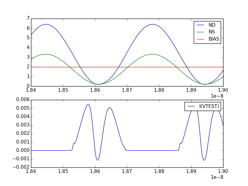
It can be shown that an increase in \(I_b\) increases the oscillation
amplitude. When the oscillation amplitude (at nd) approaches \(V_{dd}\),
a damping will appear at the middle of the current peak, because
\(V_{ds} = V_{nd}\) - \(V_{ns}\) will be near to zero. If the
oscillation amplitude increases further \(V_{ds}\) crosses 0V and becomes
negative for a small period of time. Accordingly, \(I_d\) crosses 0A and
becomes negative for such period.
Of course, in any case, the average current through M1 has to be equal to \(I_b\). In fact:
>> print(res['i(vtest)'].mean())
0.00119411417458
Which is close enough counting that it is calculated over a fractional number of periods.
During a period, M1 is always on, switching from saturation region (\(Vgs > Vt\), \(Vgd < Vt\)) to ohmic operation (channel at both source and drain). The latter happens when \(I_d\) is maximum.
