ahkab.time_functions

This module contains several basic time functions.

The classes that are found in module are useful to provide a time-varying characteristic to independent sources.

Notice that the time functions are not restricted to those provided here, the user is welcome to provide his own. Implementing a custom time function is easy and common practice, as long as you are interfacing to the simulator through Python. Please see the dedicated section Defining custom time functions below.

Classes defined in this module

pulse(v1, v2, td, tr, pw, tf, per)	Square wave aka pulse function
pwl(x, y[, repeat, repeat_time, td])	Piece-Wise Linear (PWL) waveform
sin(vo, va, freq[, td, theta, phi])	Sine wave
exp(v1, v2, td1, tau1, td2, tau2)	Exponential wave
sffm(vo, va, fc, mdi, fs, td)	Single-Frequency FM (SFFM) waveform
am(sa, fc, fm, oc, td)	Amplitude Modulated (AM) waveform

Supplying a time function to an independent source

Providing a time-dependent characteristic to an independent source is very simple and probably best explained with an example.

Let’s say we wish to define a sinusoidal voltage source with no offset, amplitude 5V and 1kHz frequency.

It is done in two steps:

• first we define the time function with the built-in class ahkab.time_functions.sin:

  sin1k = time_functions.sin(vo=0, va=5, freq=1e3)
  

• Then we define the voltage source and we assign the time function to it:

  cir.add_vsource('V1', 'n1', cir.gnd, 1, function=mys)
  

In the example above, the sine wave is assigned to a voltage source 'V1', that gets added to a circuit cir (not shown).

Defining custom time functions

Defining a custom time function is easy, all you need is either:

• A function that takes a float (the time) and returns the function value,
• An instance with a __call__(self, time) method. This solution allows having internal parameters, typically set through the constructor.

In both cases, in time-based simulations, the simulator will call the object at every time step, supplying a single parameter, the simulation time (time in the following, of type float).

In turn, the simulator expects to receive as return value a float, corresponding to the value of the time-dependent function at the time specified by the time variable.

If the time-dependent function is used to define the characteristics of a voltage source (VSource), its return value has to be expressed in Volt. In the case of a current source (ISource), the return value is to be expressed in Ampere.

The standard notation applies.

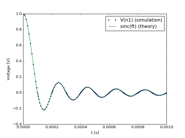
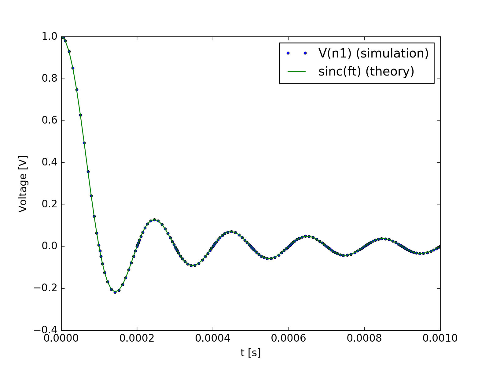
As an example, we’ll define a custom time-dependent voltage source, having a \(\mathrm{sinc}(ft)\) characteristic. In this example, \(f\) has a value of 10kHz.

First we define the time function, in this case we’ll do that through the Python lambda construct.

mys = lambda t: 1 if not t else math.sin(math.pi*1e4*t)/(math.pi*1e4*t)

Then, we define the circuit – a very simple one in this case – and assign our mys function to V1. In the following circuit, we simply apply the voltage from V1 to a resistor R1.

import ahkab
cir = ahkab.Circuit('Test custom time functions')
cir.add_resistor('R1', 'n1', cir.gnd, 1e3)
cir.add_vsource('V1', 'n1', cir.gnd, 1, function=mys)
tr = ahkab.new_tran(0, 1e-3, 1e-5, x0=None)
r = ahkab.run(cir, tr)['tran']

Plotting Vn1 and the expected result (\(\mathrm{sinc}(ft)\)) we get:

(Source code, png, hires.png, pdf)

Module reference

class am(sa, fc, fm, oc, td)

Amplitude Modulated (AM) waveform

Mathematically, it is described by the equations:

• \(0 \le t \le t_D\):

\[f(t) = O\]

• \(t > t_D\)

\[f(t) = SA \cdot \left[OC + \sin \left[2\pi f_m (t - t_D) \right] \right] \cdot \sin \left[2 \pi f_c (t - t_D) \right]\]

Parameters:

sa : float

Signal amplitude in Volt or Ampere.

fc : float

Carrier frequency in Hertz.

fm : float

Modulation frequency in Hertz.

oc : float

Offset constant, setting the absolute magnitude of the modulation.

td : float

Time delay before the signal begins, in seconds.

class exp(v1, v2, td1, tau1, td2, tau2)

Exponential wave

Mathematically, it is described by the equations:

• \(0 \le t < TD1\):

\[f(t) = V1\]

• \(TD1 < t < TD2\)

\[f(t) = V1+(V2-V1) \cdot \left[1-\exp \left(-\frac{t-TD1}{TAU1}\right)\right]\]

• \(t > TD2\)

\[f(t) = V1+(V2-V1) \cdot \left[1-\exp \left(-\frac{t-TD1}{TAU1}\right)\right]+(V1-V2) \cdot \left[1-\exp \left(-\frac{t-TD2}{TAU2}\right)\right]\]

Parameters:

v1 : float

Initial value.

v2 : float

Pulsed value.

td1 : float

Rise delay time in seconds.

td2 : float

Fall delay time in seconds.

tau1 : float

Rise time constant in seconds.

tau2 : float

Fall time constant in seconds.

class pulse(v1, v2, td, tr, pw, tf, per)

Square wave aka pulse function

Parameters:

v1 : float

Square wave low value.

v2 : float

Square wave high value.

td : float

Delay time to the first ramp, in seconds. Negative values are considered as zero.

tr : float

Rise time in seconds, from the low value v1 to the pulse high value v2.

tf : float

Fall time in seconds, from the pulse high value v2 to the low value v1.

pw : float

Pulse width in seconds.

per : float

Periodicity interval in seconds.

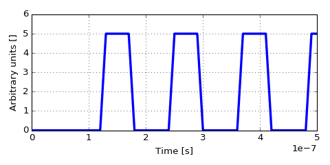
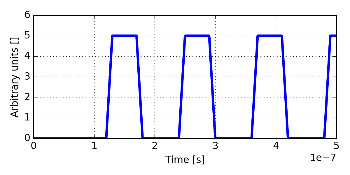
class pwl(x, y, repeat=False, repeat_time=0, td=0)

Piece-Wise Linear (PWL) waveform

A piece-wise linear waveform is defined by a sequence of points \((x_i, y_i)\).

Please supply the abscissa values \(\{x\}_i\) in the vector x, the ordinate values \(\{y\}_i\) in the vector y, separately.

Parameters:

x : sequence-like

The abscissa values of the interpolation points.

y : sequence-like

The ordinate values of the interpolation points.

repeat : boolean, optional

Whether the waveform should be repeated after its end. If set to True, repeat_time also needs to be set to define when the repetition begins. Defaults to False.

repeat_time : float, optional

In case the waveform is set to be repeated, setting the repeat flag above, the parameter, defined in seconds, set the first time instant at which the waveform repetition happens.

td : float, optional

Time delay before the signal begins, in seconds. Defaults to zero.

Example:

The following code:

import ahkab
import numpy as np
import pylab as plt
# vs = (x1, y1, x2, y2, x3, y3 ...)
vs = (60e-9, 0, 120e-9, 0, 130e-9, 5, 170e-9, 5, 180e-9, 0)
x, y = vs[::2], vs[1::2]
fun = ahkab.time_functions.pwl(x, y, repeat=1, repeat_time=60e-9, td=0)
myg = np.frompyfunc(fun, 1, 1)
t = np.linspace(0, 5e-7, 2000)
plt.plot(t, myg(t), lw=3)
plt.xlabel('Time [s]'); plt.ylabel('Arbitrary units []')

Produces:

(Source code, png, hires.png, pdf)

class sffm(vo, va, fc, mdi, fs, td)

Single-Frequency FM (SFFM) waveform

Mathematically, it is described by the equations:

• \(0 \le t \le t_D\):

\[f(t) = V_O\]

• \(t > t_D\)

\[f(t) = V_O + V_A \cdot \sin \left[2\pi f_C (t - t_D) + MDI \sin \left[2 \pi f_S (t - t_D) \right] \right]\]

Parameters:

vo : float

Offset in Volt or Ampere.

va : float

Amplitude in Volt or Ampere.

fc : float

Carrier frequency in Hz.

mdi : float

Modulation index.

fs : float

Signal frequency in HZ.

td : float

Time delay before the signal begins, in seconds.

class sin(vo, va, freq, td=0.0, theta=0.0, phi=0.0)

Sine wave

Mathematically, the sine wave function is defined as:

• \(t < t_d\):

\[f(t) = v_o + v_a \sin\left(\pi \phi/180 \right)\]

• \(t \ge t_d\):

\[f(t) = v_o + v_a \exp\left[-(t - t_d)\,\theta \right] \sin\left[2 \pi f (t - t_d) + \pi \phi/180\right]\]

Parameters:

vo : float

Offset value.

va : float

Amplitude.

freq : float

Sine frequency in Hz.

td : float, optional

time delay before beginning the sinusoidal time variation, in seconds. Defaults to 0.

theta : float optional

damping factor in 1/s. Defaults to 0 (no damping).

phi : float, optional

Phase delay in degrees. Defaults to 0 (no phase delay).

Note

This implementation is consistent with the SPICE simulator, other simulators use different formulae.