ahkab.fourier¶

This module offers the functions needed to perform a Fourier analysis of the results of a simulation.

Module reference¶

fourier(label, tran_results, fund)[source]¶

Fourier analysis of the time evolution of a variable.

In particular, the function uses the first 10 multiples of the fundamental frequency and a rectangular window.

A variable amount of time data is used, resampled with a fixed time step. The length of the data is decided as follows:

The data should be taken from the end of the simulation, so that if there is any build-up or stabilization process, the Fourier analysis is not affected (or less affected) by it.
At least 1 period of the fundamental should be used.
Not more than 50% of the total simulation time should be used, if possible.
Respecting the above, as much data as possible should be used, as it leads to more accurate results.

Parameters:

label : str or tuple of str: The identifier of a variable. Eg. 'Vn1' or 'I(VS)'. If r is your tran_solution object, calling r.keys() will give you all the possible variable names for your result set. If a tuple of two identifiers is provided, the difference of the two, in the form label[0]-label[1], will be used.
tran_results : tran_solution instance: The TRAN results containing the time data for the 'label' variable.
fund : float: The fundamental frequency, in Hertz.

Returns:

f : ndarray of floats: The frequencies correspoding to the F array below.
F : ndarray of complex data: The result of the Fourier transform, including DC.
THD : float: The total harmonic distortion. This value, for a meaningful case, should be in the range (0, 1).

spicefft(label, tran_results, freq=None, **args)[source]¶

FFT analysis of the time evolution of a variable.

This function is a much more flexible and complete version of the ahkab.fourier.fourier() function.

The function uses a variable amount of time data, resampled with a fixed time step. The time interval is specified through the start and stop parameters, if they are not set, all the available data is used.

The function behaves differently whether the parameter freq is specified or not:

If the fundamental frequency freq (\(f\) in the following) is specified, the function will perform an harmonic analysis, considering only the DC component and the harmonics of \(f\) up to the 9th (ie \(f\), \(2f\), \(3f\) \(\dots\) \(9f\)).
If freq is left unspecified, a standard FFT analysis is performed, starting from \(f = 0\), to a frequency \(f_{max} = 1/(2T_{TOT}n_p)\), where \(T_{TOT}\) is the total length of the considered data in seconds and \(n_p\) is the number of points in the FTT, set through the np parameter to this function.

Parameters:

label : str, or tuple of str

The identifier of a variable. Eg. 'Vn1' or 'I(VS)'. If r is your tran_solution object, calling r.keys() will give you all the possible variable names for your result set. If a tuple of two identifiers is provided, the difference of the two, in the form label[0]-label[1], will be used.

tran_results : tran_solution instance

The TRAN results containing the time data for the 'label' variable.

freq : float, optional

The fundamental frequency, in Hertz. If it is specified, the output will be limited to the harmonics of this frequency. The THD evaluation will also be enabled.

start : float, optional

The first time instant to be considered for the transient analysis. If unspecified, it will be the beginning of the transient simulation.

from : float, optional

Alternative specification of the start parameter.

stop : float, optional

Last time instant to be considered for the FFT analysis. If unspecified, it will be the end time of the transient simulation.

to : float, optional

Alternative specification of the stop parameter.

np : integer

A power of two that specifies how many points should be used when computing the FFT. If it is set to a value that is not a power of 2, it will be rounded up to the nearest power of 2. It defaults to 1024.

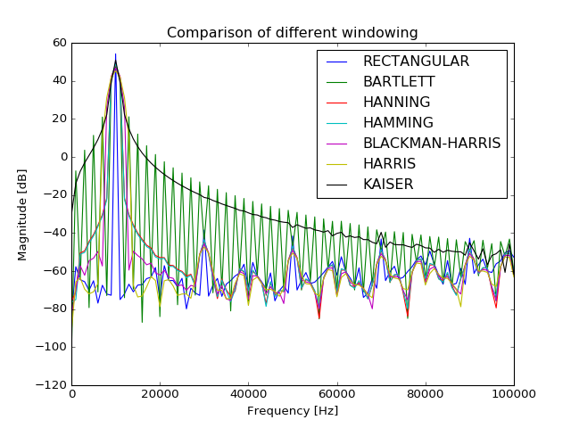
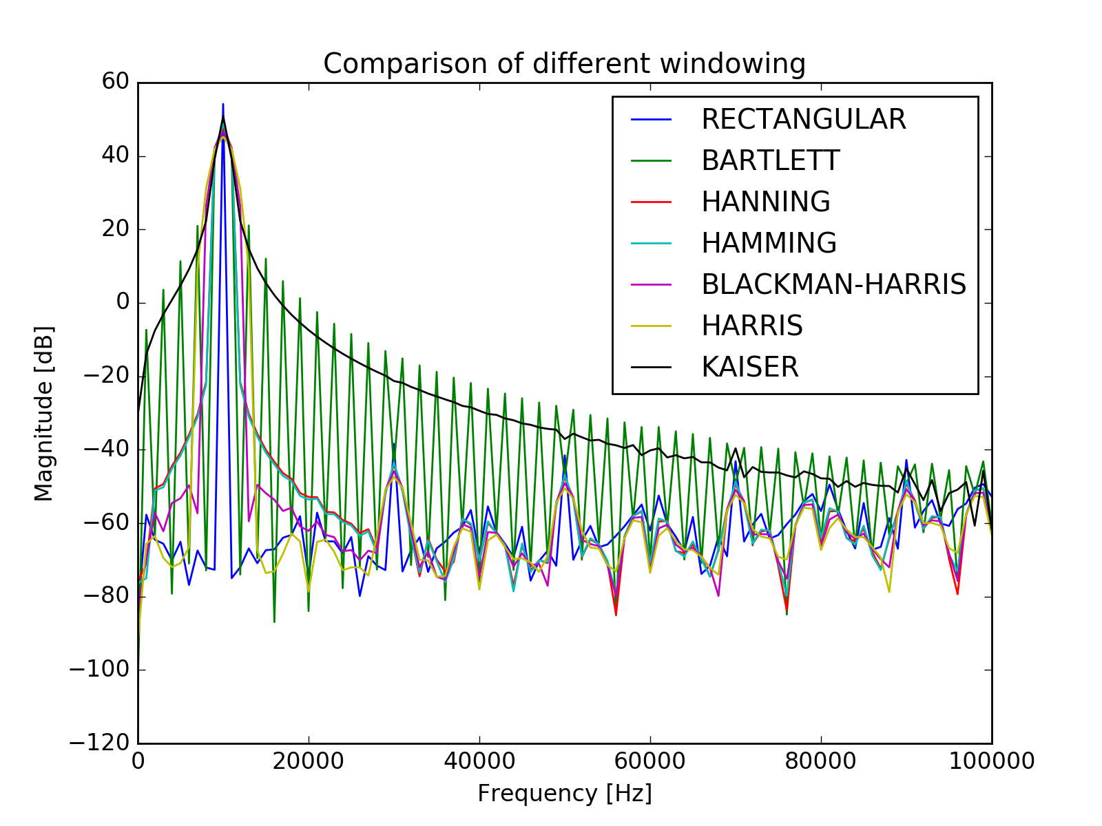
window : str, optional

The windowing type. The following values are available:

‘RECT’ for a rectangular window, equivalent to no window at all.
‘BART’, for a Bartlett window.
‘HANN’, for a Hanning window.
‘HAMM’ for a Hamming window.
‘BLACK’ for a Blackman window.
‘HARRIS’ for a Blackman-Harris window.
‘GAUSS’ for a Gaussian window.
‘KAISER’ for a Kaiser-Bessel window.

The default is the rectangular window.

alpha : float, optional

The \(\sigma\) for a gaussian window or the \(beta\) for a Kaiser window. Defaults to 3 and is ignored if a window different from Gaussian or Kaiser is selected.

fmin : float, optional

Suppress all data below this frequency, expressed in Hz. The suppressed data is neither returned nor used to compute the THD (if it is computed at all). The DC component is always preserved. Defaults to: return and use all data.

fmax : float, optional

The dual to fmin, discard data above fmax and also do not use it if computing the THD. Defaults to infinity.

Returns:

f : ndarray of floats: The frequencies, including the DC.
F : ndarray of complex data: The result of the Fourier transform, including DC.
THD : float: The total harmonic distortion, if freq was specified, None otherwise.

(Source code, png, hires.png, pdf)